Explain me the sampling method
by Valentin Stefan - last update 11 December 2019
One iteration
Explain
Consider theSafariland web from the bipartite package, which looks like this:
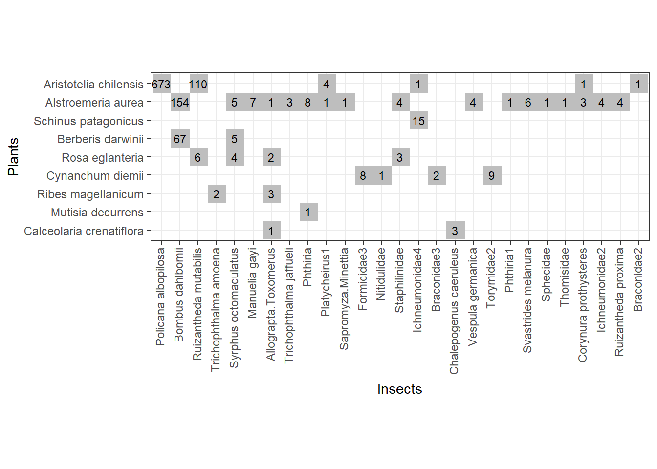
Fig. 1 - Safariland web from which we will sample without replacement
There are 1130 total interactions in the web. We can draw the first start sample of, say, 100 random interactions without replacement.
Side note: for a start value of 100 interactions and a step of 50, the sampling procedure splits the 1130 interactions into 21 sub-webs (first one contains 100 interactions, then each subsequent one contains approximatively 50 more sampled interactions on top of the previous one).
So, with the start sample of 100 interactions we can form this web below (Fig 2). All names of plants and insects are kept for easy visual comparison with the entire web from above (Fig 1).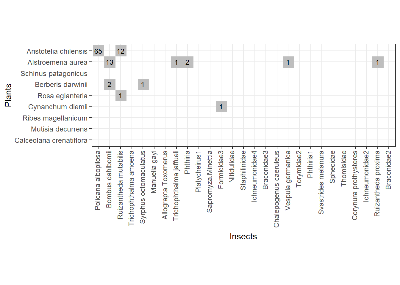
Fig. 2 - The web formed with the first sample of interactions from Safariland
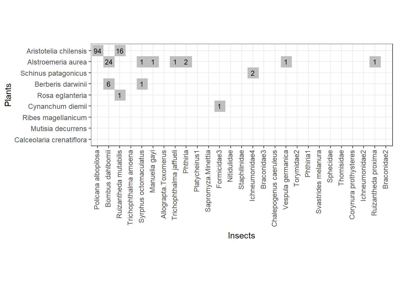
Fig. 3 - The web formed with adding the second sample of interactions from Safariland
Note that, in the second sub-web we managed to sample new species by sampling 50 more interactions:
- higher level species (OX axis): Ichneumonidae4, Manuelia gayi
- lower level species (OY axis): Schinus patagonicus
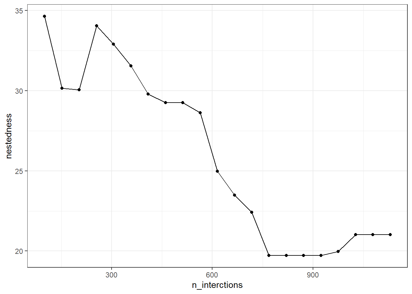
Fig. 4 - Nestedness values for each sampled web. The last value corresponds to the entire Safariland web
Animation
Below is an animation of the sampling method (one iteration):

Multiple iterations
If we repeat this sampling procedure n times, then we get n lines. We can then compute an average line with 95% quantile based confidence intervals as in Fig. 5 below.
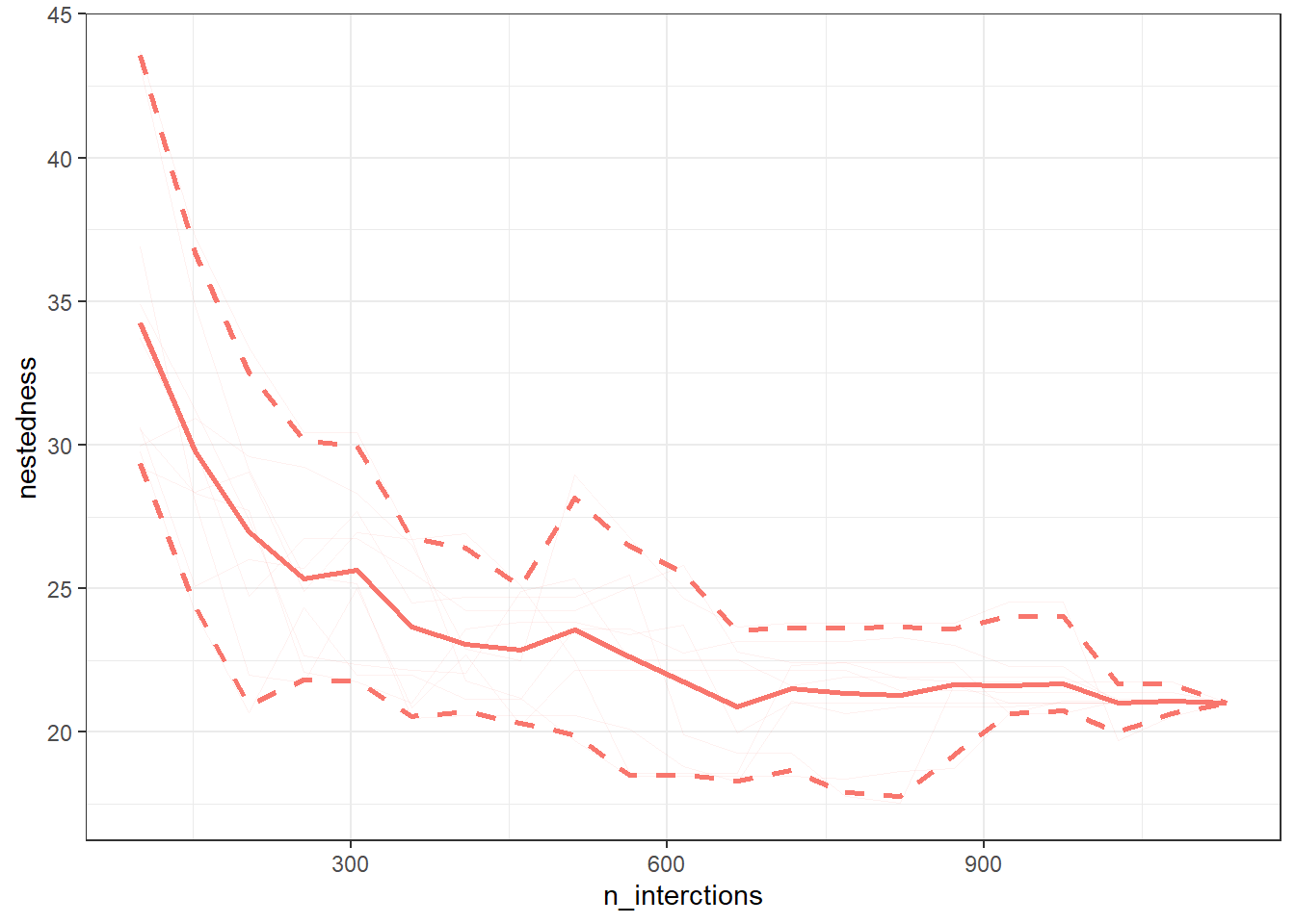
Fig. 5 - Sampled nestedness values, 10 interations. The thick continuous line represents the average line and the dashed lines depict the 95% quantile based confidence intervals around the mean line.
Such accumulation/rarefaction curves allow comparison of networks/webs with different number of interactions. Ideally the indices/metrics will be compared if the curves display a trend of reaching an asymptote. That means that if we keep on investing effort to sample interactions (observe plant-pollinator in the field) we will not gain much further information, so network comparison is already possible.